
486 Final Project
Can we predict the total casualties (injuries and deaths) based on the time the accident happens?
Introduction
Before I even started playing with any data I was questioning my choice to go with this question as it could be viewed as somewhat morbid. However, my reasoning is to try and see if these events are predictable. IF they turn out to be based on the methods I’ll be employing then arguments could be better made for the prevention of these events. In my mind this is something that could be very valuable to any city or town wanting to reduce accidents that result in injury and death. The complexities involved in these accidents necessitate comprehensive study to find patterns, mitigate risks, and enhance safety measures. I would also like to mention that the analysis in this post is only a small fraction of knowledge that can be gained from this type of information. There are almost 30 different variables in this dataset that could also be considered to answer many more questions regarding motor vehicle accidents.
The use of multiple machine learning models is very important in offering a comprehensive exploration of the data, enhancing predictive accuracy, providing interpretability, and shedding light on the relationships between all the variables in this dataset, which I why I mentioned just earlier the recognition that there is so much more that can be done. Here is the link to the Github repository that contains all the code for the work that was performed.
The Work
Cleaning the data necessary to answer this question was a simple task of creating features for the individual aspects of each crash’s timestamp.
data['CRASH DATE'] = pd.to_datetime(data['CRASH DATE'])
data['CRASH TIME'] = pd.to_datetime(data['CRASH TIME'], format='%H:%M')
data['Hour'] = data['CRASH TIME'].dt.hour
data['DayOfWeek'] = data['CRASH DATE'].dt.dayofweek
data['Month'] = data['CRASH DATE'].dt.month
Along with these features our target variable was created using the sum of all injuries and fatalities:
data['Total Casualties'] = data['NUMBER OF PERSONS INJURED'] + data['NUMBER OF PERSONS KILLED'] + data['NUMBER OF CYCLIST KILLED'] + data['NUMBER OF CYCLIST INJURED'] + data['NUMBER OF MOTORIST INJURED'] + data['NUMBER OF MOTORIST KILLED'] + data['NUMBER OF PEDESTRIANS INJURED'] + data['NUMBER OF PEDESTRIANS KILLED']
features = ['Hour', 'DayOfWeek', 'Month']
target = 'Total Casualties'
It is important to note that I chose not to drop the rows where the total casualty count was zero. Removing rows with zero total casualties might improve the model’s ability to predict cases involving injuries or fatalities by reducing noise or instances where injuries/deaths didn’t occur. But on the other hand, removing these rows could lead to a reduction in the dataset size, potentially losing valuable information that would contribute to intepreting the results of the question.
The first model is just a basic one:
model = RandomForestRegressor(n_estimators=100, random_state=42)
model.fit(X_train, y_train)
This model had an MSE of 0.4838 which means that on average the squared error between the actual and predicted values was only about 0.5. Which I thought was pretty good. I then fit the model again using grid search to see which hyperparamers would be the best to use in building the model.
param_grid = {
    'n_estimators': [50, 100, 150],
    'max_depth': [None, 5, 10, 15],
    'min_samples_split': [2, 5, 10],
    'min_samples_leaf': [1, 2, 4]
}

rf = RandomForestRegressor(random_state=42)
grid_search = GridSearchCV(estimator=rf, param_grid=param_grid, cv=5, scoring='neg_mean_squared_error', n_jobs=-1)
grid_search.fit(X_train, y_train)
As an interesting fact, the first model took about a minute to train, but with Grid Search it took an hour and a half. I should also mention that this is the first time that I had worked with a dataset of this size, even though I was only using 3 or 4 features from it.
To my dismay the MSE didn’t really improve after finding that the best model. I thought about this and realized that in the creation of my features I had accidentally used the ‘Crash Date’ column to make the ‘Hour’ variable. Crash Date did not have any time information so the Hour variable was all zero’s. I fixed this and then ran both models again. With the first basic model the MSE went to 1.92. and the results of grid search weren’t much different.
Best Model Mean Squared Error: 1.9254814342085336
Best Parameters: {'max_depth': 10, 'min_samples_leaf': 1, 'min_samples_split': 2, 'n_estimators': 150}
Again, no change.
Using grid search, although being a powerful technique for hyperparameter optimization, confronts inherent limitations that could contribute to its very similar MSE with the baseline model. Firstly, while grid search thoroughly explores hyperparameter combinations within predefined ranges, it operates under the constraint of computational resources, which can restrict the exploration space and hinder the discovery of the right hyperparameters beyond the specified grid. Also, grid search might inadvertently overlook interactions between hyperparameters or fail to capture some nuanced model behaviors, leading to a convergence towards non-optimal configurations despite the comprehensive search. Additionally, the dataset’s complexity and noise might limit the discernibility of performance improvements made through hyperparameter tuning, which results in minimal differences in MSE between the grid search model and the baseline model.
Lastly, the dataset’s characteristics, such as the distribution of accidents, temporal patterns, or subtle dependencies between features, might impose limitations on the models’ predictive capabilities, thus constraining large improvements on MSE even after tuning the typerparamers. These factors collectively contribute to the converging of MSE values between the grid search model and the baseline, emphasizing the need for a more holistic approach considering the model’s limitations, dataset nuances, and exploration of other modeling methodologies beyond hyperparameter tuning.
Lastly I decided to apply an unsupervised learning method to try and indentify any other patterns in the dataset. Using K-means clustering by the hour of the day I produced the following graphic:
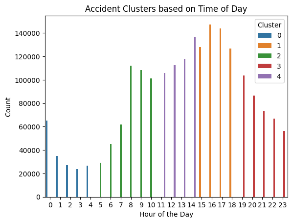
As you can see, the clusters with the highest peaks are from 11am - 2pm and about 3pm - 6pm. While this is just a basic cluster graphic, I believe its a good thing that it is also somewhat intuitive. This tells me not only that the data is good, but also that the model is good because it follows what I would expect to see from crash data. Higher activity into the afternoon and evening, and then dropping way down in the very early hours of the morning when much less people are on the roads.
Conclusion
In conclusion, while I encountered challengers interpreting the initial models, there is still plenty of room for exploration and analysis in this dataset. The initial modeling endeavors, though not very successful offered valuable glimpses into the complex nature of accidents. However, the dataset’s complexities and other characteristics surpassed my interpretability of the model. Despite these limitations, the dataset’s potential is obvious, primarily evident in the K-means cluster graphic. This graphic, depicting distinct temporal patterns and clusters of accident occurrences across hours of the day, underscores the dataset’s richness and versatility . The peaks and divergent clusters hint at nuanced temporal trends that call for more exploration and model refinement. Further exploration should focus on harnessing the wealth of this data, refining modeling techniques, and deploying more interpretable models to see the intricacies.